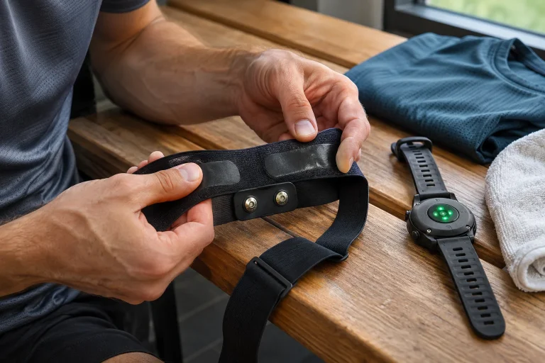
Your run’s heart-rate graph is a neat, continuous line, and the exported table contains one number per second. Calculating beat intervals from these and then performing your own HRV analysis may seem an obvious idea. The problem is that displayed heart rate may already be summarised data. It does not necessarily preserve exactly when each heartbeat occurred.
HRV concerns variation in the time between beats, so it requires different information from average beats per minute. This article unpacks the data-chain distinction: what an RR time series means, why it cannot be restored from a smoothed curve and what to look for in a sports-watch export. The short original examples are purely mathematical illustrations; they do not indicate health, illness or readiness to train.
Beats per minute is not a list of every beat’s time
If the number of beats and duration of a window are known, an average frequency can be calculated. That does not show how beats were distributed within the window. The same number of events can occur evenly or at alternating intervals. An average compresses total time and event count, discarding some details of order. Another formula cannot undo this information loss afterwards.
The Kubios HRV Scientific 2026 user guide explicitly distinguishes beat-to-beat intervals from heart-rate values averaged over periods. Average heart rate given every one or five seconds cannot substitute for genuine beat-interval-based HRV analysis. What matters is not table density, but which events produced the numbers.
In the first version of our original four-second example, four successive intervals are 1000, 1000, 1000 and 1000 milliseconds. In the second they are 900, 1100, 900 and 1100. Both total four thousand milliseconds and have an average interval of one thousand. The equal-length series contain the same number of intervals, while every successive value differs in the second. The sum does not reveal that difference.
An RR series preserves successive intervals
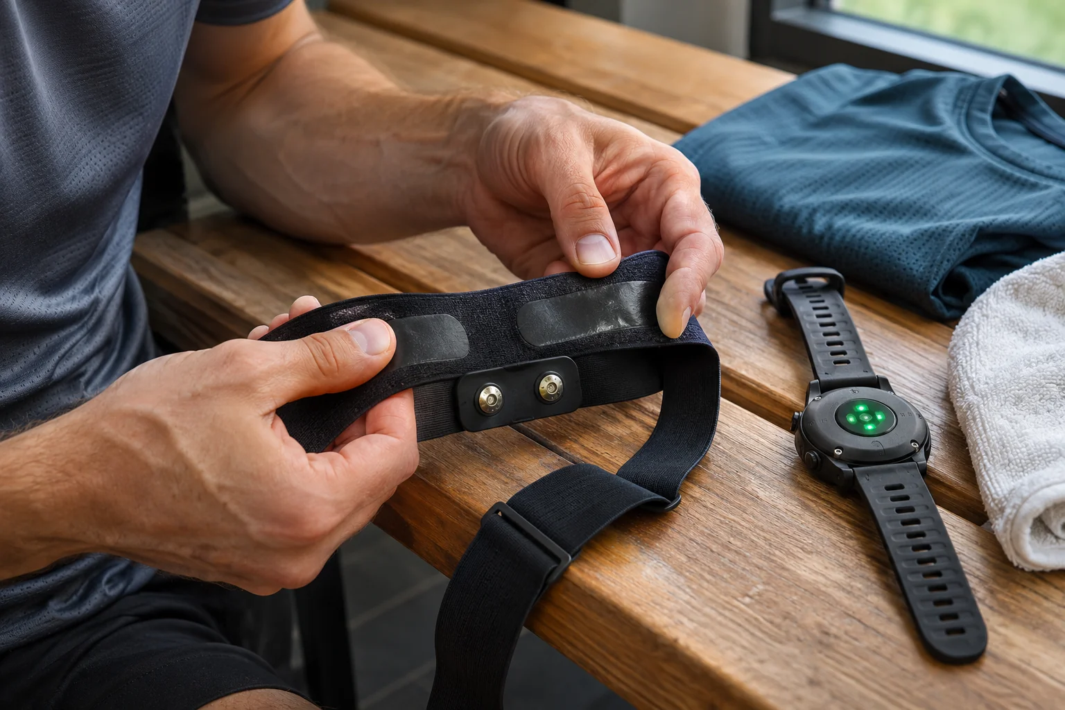
RR refers to the time between characteristic R waves in an ECG. An interval series can describe how many milliseconds passed from one detected heartbeat to the next. This differs from a complete ECG voltage–time trace and from beats per minute. Storing one does not automatically make the others available in the same export.
The official Garmin FIT Activity documentation describes arrays of RR intervals in separate HRV messages. A normal Record message’s heart-rate field and these intervals are different things. The format can carry the appropriate information, but that does not mean every watch’s activity file actually contains it. Check the specific recording and export chain.
It is also useful to distinguish detected intervals from the series of normal beats accepted for analysis. A wrongly detected signal or another phenomenon does not automatically become appropriate HRV data because a number appears in a table. Signal origin, acceptance rules and documented processing are parts of analysis. “Raw data” does not inherently mean error-free data.
Why can RMSSD differ with the same average?
RMSSD is the square root of the mean squared differences between successive intervals. The Kubios guide also provides this definition. More simply, it summarises changes between neighbouring intervals and is expressed in units of time. It is not the average interval, the standard deviation of heart rate or the difference between the highest and lowest heart rates of a whole run.
The earlier original constant four-value series has three adjacent differences of zero, so its illustrative RMSSD is zero too. The differences in 900–1100–900–1100 are +200, −200 and +200 milliseconds. Each square is 40,000, their mean is 40,000 and its square root is 200. The same average interval therefore occurs in this artificial example with either zero or two hundred milliseconds.
A four-value series is not a real measurement protocol, and we attach no physiological judgement to the results. It shows that adjacent changes cannot be uniquely calculated from the average. If only the one-thousand-millisecond mean survived, we cannot determine which series produced it. What restoration lacks is lost information, not merely a well-chosen calculator.
 Enlarge image
Order matters too, not only the set of values
Rearrange our second series into 900, 900, 1100 and 1100 milliseconds. It contains the same two smaller and two larger numbers, with unchanged average and sum. Adjacent differences are now zero, two hundred and zero. Their mean square is 40,000/3 and its square root about 115.5 milliseconds. This differs from two hundred in the alternating order.
A sorted frequency table therefore does not necessarily preserve all information needed for calculation either. Knowing only how often an interval occurred, but not original order, loses some adjacent changes. Temporal order is data in an RR series. Do not load intervals into analysis software sorted by value.
Directly joining across a missing section can also change adjacency. If you simply put two separate recording sections together, the join can create a neighbouring pair that was not two successive beats in reality. Marking gaps and handling analysis windows therefore matter. A tidy-looking table does not guarantee a temporally continuous, interpretable signal.
The reciprocal formula works only with appropriate input
For a single known interval, 60,000 divided by its duration in milliseconds assigns a frequency. One thousand milliseconds corresponds to sixty events per minute. That does not make the complete interval sequence behind averaged heart rate recoverable. The formula transforms one number into another; it does not invent original timings already combined.
In an original example, 900 and 1100 milliseconds correspond to about 66.67 and 54.55 events per minute. Their simple arithmetic average is around 60.61, while the reciprocal of the one-thousand-millisecond average interval gives sixty. Reversing averaging and taking the reciprocal can therefore produce different results. This is a mathematical property, not a brand’s unusual behaviour.
When software creates an “RR” column from every-second heart rate, check what it calls RR. It may be a converted duration associated with average heart rate, rather than the original spacing of detected beats. A column name does not validate input on its own. Without distinguishing a genuine event list from an approximation derived from a pulse curve, the resulting HRV can look misleadingly precise.
Smoothing and rounding leave no unique route back
A moving average or other smoothing can deliberately reduce some short-term variation for display. This may help create a readable heart-rate graph, but differs from preserving every beat’s exact timing. If several original series lead to the same smoothed curve, none can be selected with certainty from that curve. A prettier line does not automatically contain omitted detail.
In an original rounding example, 999 and 1001 milliseconds correspond to about 60.06 and 59.94 events per minute. Rounded to whole numbers, both are sixty. Converting those rounded sixties back produces one thousand milliseconds every time and removes the original two-millisecond alternation. Displaying more decimal places afterwards cannot restore that lost detail.
An every-second file row does not necessarily represent one beat either. At a higher heart rate, several beats can occur within a second; at a lower rate, events may fall differently across window boundaries. Recording cadence and heartbeat event times are different concepts. Do not therefore automatically calculate detected beat count from the number of data points.
Artifacts may alter HRV more than the average
Bourdillon and colleagues’ original 2022 study examined error effects in athletes’ interval series with artificial modifications and natural artifacts. Results indicated that RMSSD can be sensitive to these deviations even when average heart rate changes less. The study’s specific thresholds are not general home acceptance limits; the message concerns data quality.
In an original technical example, a system returns two actually one-thousand-millisecond intervals as one two-thousand-millisecond interval because it missed an event. Total elapsed time can remain approximately correct while interval order and adjacent differences change. The two-thousand value does not prove such a long beat interval actually occurred. Distinguishing detection error from a physiological event requires suitable signal and expertise.
Repair is not simply deleting every unusual value until the graph looks pleasant. Automatic filtering applies assumptions and can alter the result. Preserve the original, correction method and affected section markings. If a recording cannot support reliable analysis, indicating missing data or uncertainty is more informative than an attractive but unsupported HRV value.
 Enlarge image
What does an actual device comparison show?
In Johansson and colleagues’ observational study published in January 2026, ECG, a Polar H10 chest strap and a phone-camera app were compared in 37 trained participants using repeated same-day recordings. Under that protocol, the chest strap showed smaller deviations from ECG than the camera method studied. This concerns a specific brief measurement situation, not a general rating of every wrist measurement during running.
The point is that such validation examines suitable event or signal data and a comparison procedure. It does not establish that an artificial series reconstructed from averaged heart rate is equally suitable. Nor does a device name in a source automatically make a file recorded with another app and export setting identical in content. Device, app, protocol and processing matter together.
An ECG function’s name does not itself imply diagnostic authority either. The Polar information on its own wrist ECG, for example, explicitly states the function’s non-medical, non-diagnostic purpose. Interpreting an athlete’s interval or HRV data must not be confused with diagnosing an arrhythmia. A training-log number belongs to measurement and training context; alone, it is not a clinical examination result.
Export checks: identify the data type first
First ask whether you received actual beat intervals or heart rate summarised at intervals. Check device and exporter documentation, field names and units. Milliseconds and seconds differ a thousandfold, while a timestamp is not the same as the time between two beats. One wrong unit can produce an entirely different magnitude.
Second, record the section analysed and its circumstances. Series collected at rest, during running and during sleep have different contexts. Your own log can include posture, recording start, duration, device and reported gaps as separate fields. This metadata helps determine whether two results are comparable. Even identical names can conceal different measurement contents.
Finally, keep the raw source and analysis settings. If only a smoothed heart-rate curve remains, do not retrospectively create a series labelled genuine beat intervals from it. Missing information can be acquired through a new appropriate recording, not inserted retroactively into the original. The useful technological decision is clarifying data type: a later HRV value can then summarise the phenomenon for which measurement data actually exists.
Sources
- Kubios HRV Scientific 2026: supported data and HRV parameters.
- Garmin FIT Activity: HRV messages containing RR intervals.
- Bourdillon and colleagues, 2022: artifact effects on HRV parameters.
- Johansson and colleagues, 2026: simultaneous device HRV validation in athletes.
- Polar: the intended purpose of wrist ECG.
How Futószív articles are prepared: our editorial guidelines.