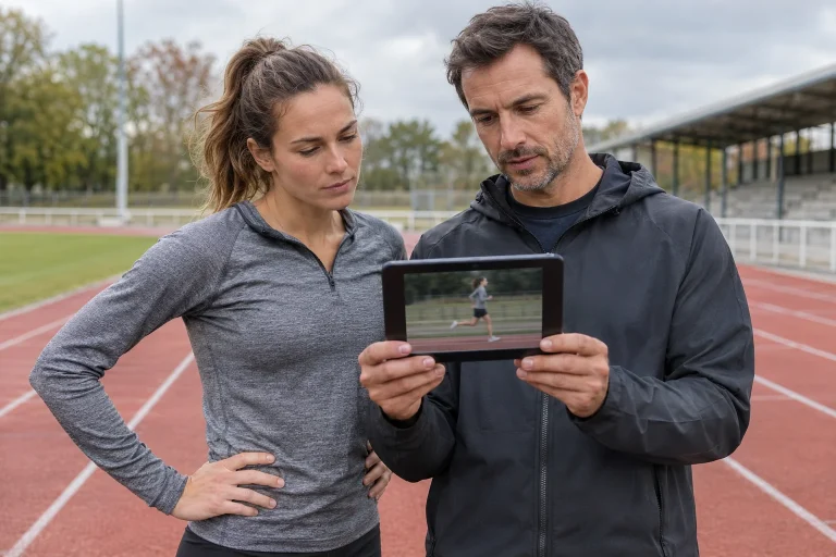
A colourful flow diagram contains a runner surrounded by blue and red vortices. It looks detailed, but the first question is not how powerful the computer is. It is whether the runner actually moves. One fixed pose, several separately frozen positions and a person moving over time present three different tasks to the air.
Simplification is not itself an error. A stationary model can answer many well-defined questions usefully. Problems begin when a fixed-body calculation is presented as complete evidence for a moving person. We explain what to look for in methods, what a checked calculation means and how real airflow measurements around runners can complement models.
A stationary figure is not the same as a person running at constant speed
A runner’s torso can travel at nearly constant average speed while arms and legs continually accelerate, slow and change direction relative to it. Different body parts therefore have different instantaneous speeds relative to air. A fixed mannequin or digital body omits that relative movement if every surface stays unchanged relative to the flow.
In our kinematic example, the torso travels at four metres per second relative to the ground in still air. An imaginary hand momentarily swings forwards at one metre per second relative to the torso, making its ground speed five. Moving backwards at the same relative speed makes it three. These are not measured typical arm-swing values; they illustrate adding velocities. The fixed model has no such difference.
Conditions around the supporting and swinging legs can differ too. From a runner-moving viewpoint, the ground moves backwards; ground-related contact gives a different boundary condition from a body simply placed in air. Researchers must choose a frame of reference and treatment of the ground. This cannot be inferred from the finished image’s colours.
Three model types permit three different kinds of claim
One static pose is the simplest geometry to fix. A researcher may place the same body in different group positions and ask how arrangement changes calculated force. Posture deliberately remains constant to isolate the variable. Results concern that pose and its flow conditions.
Schickhofer and Hanson’s 2021 work investigated drag using a fixed female runner model and different formations. Beaumont and colleagues’ research on line positions also used CFD for defined geometric arrangements. Comparing formations or positions is meaningful, but is not the same as directly reproducing every moving part across a complete stride cycle.
The quasi-static approach, using several frozen poses, can show different cycle shapes. Yet each may still be treated as a separate stationary geometry. A genuinely dynamic model moves surfaces over time and connects the flow’s history to the next position. Many still images can therefore offer more information than one, but do not alone constitute a physically moving film.
 Enlarge image
Averaging snapshots also requires time weighting
If force is calculated separately in several poses, an average needs the time each represents. In our artificial example, force is six newtons in one phase and ten in another. If each occupies half the cycle, the arithmetic mean is eight newtons. If the six-newton phase occupies three quarters and the ten-newton phase one quarter, the time-weighted mean is seven.
The difference is not a new aerodynamic discovery: we averaged the same invented force values using different durations. Several attractive diagrams and two force values do not yet determine the cycle’s average demand. Selecting phases, their durations and how they are linked are parts of the method.
Actual dynamic flow can complicate matters further. A flow structure created in one pose does not necessarily disappear immediately when an arm changes position. Independently calculated states can omit precisely that temporal connection. Required detail depends on the desired result: a rough comparison, precise cycle average or time-varying effect on another runner.
What did airflow measurements around a genuinely moving runner add?
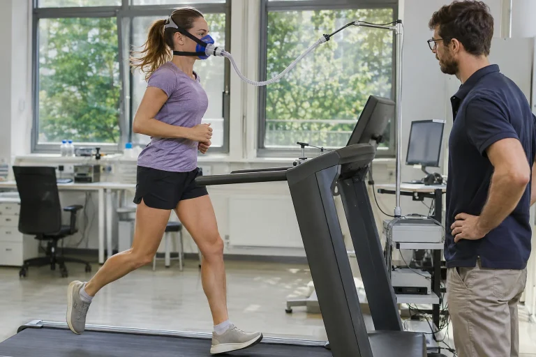
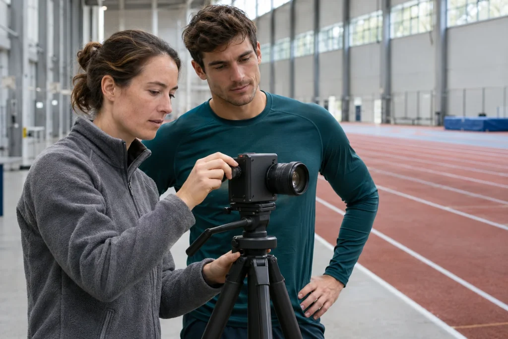
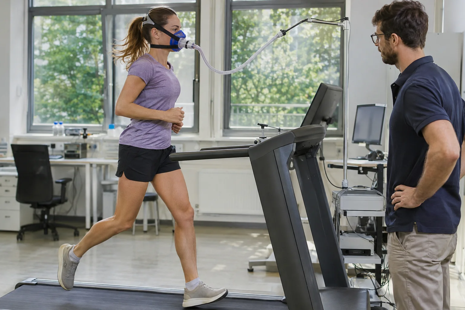
The 2026 original study On-site investigation of running aerodynamics examined six Dutch subelite junior runners in an indoor sprint hall at approximately eight metres per second. Cameras tracked helium-filled soap bubbles under LED illumination, and time-varying flow data were processed. This measured moving people within a defined sample and environment.
The analysis described near-wake asymmetries linked to limb positions; farther away, precise instantaneous posture had a less distinct influence. Importantly, the flow behind runners was measured. Possible drafting benefits calculated from it were not direct oxygen-uptake measurements in a second runner. Measured flow and the application inferred from it remain two steps.
The lesson is that field measurement and models can help differently. Measurement can check the flow characteristics behind a moving body, while calculation can vary individual parameters precisely. You need not choose between them as though only one were valuable. Strongest conclusions arise when they can be compared using the same quantities and appropriate conditions.
Why does the computational mesh matter?
CFD divides a continuous spatial problem into many computational cells. Cell size and placement affect which details the solution can resolve. The NASA technical guidance on grid convergence therefore examines changes across successively refined meshes. The important question is not simply cell count but how sensitive the quantity of interest remains to further refinement.
In our illustrative sequence, a model gives eight newtons on a coarse mesh, 7.5 on a medium mesh and 7.4 on a finer one. The shrinking change may suggest reduced sensitivity to further spatial detail. These three fictional points establish no formal error bound. They do show why ‘we used millions of cells’ is not enough in a presentation.
Refining the wrong place can add computation with little meaningful improvement. If important details near the body remain unresolved, adding density far away does not necessarily fix them. Mesh quality and problem structure matter together. Seek methodological evidence behind a result rather than the largest technical-size figure.
Time step and turbulence model check different things
Time-dependent calculations follow events in time steps. In our example, an imagined half-second cycle divided into one hundred points gives five-millisecond steps; five hundred points gives one-millisecond steps. A denser sequence may allow more temporal detail, but does not itself establish accuracy. Check how much the important result changes when the step is reduced further.
Turbulence treatment is a separate modelling choice. Not every vortex is represented at the same detail, and an approximation may work better for some flows than others. The NASA guidance on error sources distinguishes physical-model approximation from spatial and temporal discretisation error. Reducing one does not automatically remove the other.
A calculation can therefore be beautifully stable yet physically incomplete. Solving the same simplified stationary body ever more finely approaches a solution for that body. More cells alone do not restore actual arm movement. Judge accuracy separately against both the selected model and the original real-world question.
 Enlarge image
Checking the calculation and comparing it with reality are separate tasks
The NASA verification and validation framework separates solving the chosen mathematical problem correctly from how well that problem describes the reality studied. The former involves convergence and numerical procedures; the latter needs appropriate experimental or other credible reference data. These support each other but neither replaces the other.
In our imaginary project, calculation gives 7.4 newtons and a matching measurement gives 7.5 with known uncertainty. That may be a favourable comparison for that body and condition. Introducing another body, crosswind and moving limbs does not automatically extend the original agreement to every new situation. Validation has an application range.
Compare the same quantity. Good agreement in local velocity fields matters but does not necessarily imply equal accuracy for every force component. Agreement in total drag likewise does not prove every wake detail correct. Ask precisely which quantity was checked and under what conditions.
Five questions beside an impressive diagram
First: does the body have one fixed pose, several frozen phases or actual movement? Second: how are the ground and body-relative airspeed treated? Third: is mesh sensitivity and, where necessary, time-step sensitivity shown? Fourth: which measurement was used to compare the quantity of interest? Fifth: does the conclusion concern force, total energy or an already derived race time?
Read the colour scale too. The same blue in two diagrams need not mean the same airspeed if scales differ. A striking red patch may show one selected instant or plane, not directly depict force on the entire body. Good scientific visualisation names scale, plane and averaging. Without them, appearance can suggest more certainty than the data provide.
The challenge of moving people is therefore not solved by calling stationary models ‘bad’. Match simplification to the question, verify the calculation and compare it with appropriate real data. Runners benefit by recognising the evidence type behind an impressive image. Real detail is not the number of colours, but a method traceable through to its conclusion.
Sources
- D’Angelo and colleagues, 2026: field airflow measurements around moving runners.
- Schickhofer and Hanson: CFD analysis of defined body models and formations.
- Beaumont and colleagues: CFD model of line positions.
- NASA: grid convergence.
- NASA: modelling and numerical error sources.
- NASA: CFD verification and validation.
How Futószív articles are prepared: our editorial guidelines.